Gaussian Mixture Models for Clustering

If intelligence was a cake, unsupervised learning would be the cake, supervised learning would be the icing on the cake, and reinforcement learning would be the cherry on the cake. – Yann Lecun.

CONTENTS:

• Motivation

• What is Clustering?

• What are Mixture Models?

• Gaussian Mixture Model (GMM)

• Expectation-maximization Algorithm

• Working Example in Python

• How do we select the value for K?

• Applications

• References and Additional Resources

In this article, we’ll study a popular statistic model – Gaussian mixture model (GMM) and see how it can be readily applied for the unsupervised task of clustering. We’ll look at what these models are, and how they work both mathematically as well as “Pythonically”. So, before we begin, what’s our motivation to study these models?

Figure 1: R136, a prototype super star cluster

MOTIVATION

Do you know the central limit theorem? If you don’t, it simply states that if we have a population with some mean µ and standard deviation σ, and if we randomly take out a large enough sample (generally, of size > 30) from that population, then the distribution of the sample tends to be normally distributed a.k.a. Gaussian. Mathematically, Gaussian distribution is defined as:

Typically, f(x; µ, σ²) is also denoted by N(µ, σ²). If we were to plot the standard Gaussian distribution (µ = 0 and σ = 1), it would look like the one shown in the figure below.

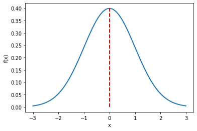
Figure 2: Standard Gaussian distribution

Furthermore, as we increase the size of samples, distribution will only converge more towards normality. A great thing about this theorem is that it will stay true no matter what the individual probability distribution of the population is! So, indeed, we take this simplistic assumption that our real-world data can be modeled using Gaussian distribution as well. However, this assumption also seems rather too restrictive and doesn’t make sense intuitively: data is not always unimodal i.e. its distribution does not always only have single-mode value or single peak value. Then, what can we do to model the multimodal data (Data with more than one mode values)? We cannot use Gaussian distribution with one peak as it will be a really poor representation of the data. Now intuitively, it will be sensible of us to say that we can use multiple distributions, each representing separate unimodal data samples and then somehow combine them to represent the multimodality in the population’s distribution. And, this is exactly what’s done. We mix the models to create a new form of model which as we’ll see are called mixture models. Before jumping into how GMMs are exploited for clustering, let’s briefly look at some of the terms in more detail. First of all, what do we mean by clustering? WHAT IS CLUSTERING?

Clustering means grouping. We take different items with different properties and assign them to a group based on their properties. In machine learning, problems like clustering come in the domain of unsupervised learning. Unsupervised means that we have no prior knowledge of to which group the item belongs to so grouping is done purely based on properties (popularly called features). As we know, in real-world, we’ll mostly encounter the data which is not labeled so tools that can help with clustering can be beneficial in many applications such as data analysis, customer segmentation, recommender systems, search engines, image segmentation, semi-supervised learning, dimensionality reduction, and many-many more.

So, now that we know what we will be using GMMs for, let’s formally define mixture models. WHAT ARE MIXTURE MODELS?

Mixture models are a simple strategy of combining probability distributions to create a richer distribution. Why do we do this? As we discussed, assuming that the data has been sampled from mixture models helps us represent the probability distribution for multimodal data. Assume we observe X1, X2, ..., Xm data values and that each has been sampled from a randomly picked jth mixture component which is one of the K mixture components. Mixture components are nothing but the groups or clusters and these terms can be used interchangeably. For example, if we want to divide people into three age groups, let’s say, children, adults, and seniors, then our mixture components will simply be {children, adults, seniors}. With a mixture component, we associate a cluster probability ϕʲ which is the probability of choosing that particular cluster. We can also say that ϕʲ represents the probability that belongs to the jth mixture component. This implies:

The index of the cluster chosen for the Xi is stored in z(i). So, when z(i) = j, we say that Xi has been randomly sampled from the jth mixture component. Often times, unlike Xi we don’t observe z(i) directly, i.e., we don’t have any information about the groups that the instances belong too. In the case of age group example, we don’t know what the age groups are. So, sometimes we call these unknown variables as latent variables.

From the law of total probability, the marginal probability for Xi will be:

GAUSSIAN MIXTURE MODEL (GMM)

When data is modeled as a mixture of components where each component is modeled as a Gaussian distribution, we call the resultant model GMM. In GMM, we assume that the instances were generated from a mixture of Gaussian distributions whose parameters are unknown. What are our parameters in this case? As we saw in the equation for Gaussian distribution, the shape of the distribution changes w.r.t two parameters: mean µ and standard deviation σ, so these are very much qualified to be our parameters. Note that standard deviation and covariance matrix Σ are responsible for describing the same kind of properties, hence we can say for GMMs, if z(i) = j, then Xi ~ N(µ(j), Σ(j)). Secondly, we saw that we have weights associated with each jth cluster as ϕʲ. These weights are unknown too. With all this, we are also assuming that all the instances from a single Gaussian distribution form a single cluster which makes sense at this point and will also be the basis of the clustering process. So, given the values for Xi for i = 1, ..., m, if we can estimate the unknown parameters for different Gaussian distributions, our objective of dividing the instances into clusters will be achieved subsequently. This whole process, by the way, of estimating the parameters for the model, given X, is accomplished by maximizing a function called likelihood function. And the process of maximizing is called maximum likelihood estimation. So now, we have an unknown parameter set θ = {µ(1), ..., µ(K), Σ(1), ..., Σ(K), ϕ¹, .., ϕᵏ}. We just have to find an appropriate likelihood function L which as a result would give us the best estimations for these parameters, and our job will be done. For this, we have Expectation-maximization (EM) algorithm. EXPECTATION-MAXIMIZATION ALGORITHM

In short, in the EM algorithm, the parameters are first initialized randomly, then we repeat two steps until convergence i.e. until we have found the values of parameters that maximize the likelihood function or log-likelihood function (one and the same thing). The first step is called Expectation where we assign instances to the clusters and the second step is Maximization where we update the clusters (i.e. update our parameter set θ). Let’s now see these two steps in-depth: Expectation step: For each Xi, where i ∈ {1, ..., m}, calculate rᵢₖ as:

Where rᵢₖ is the probability that Xi has been generated by a kth mixture component. rᵢₖ is also sometimes referred to as responsibility. Maximization step:

• Calculate total weight Wₖ (fraction of total instances assigned to mixture component) as:

• Using Wₖ, update the values for parameters of kth mixture component as:

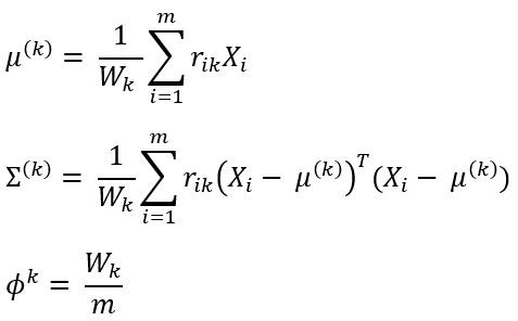
Both of these steps are repeated until the log-likelihood function L (defined below) of the model converges.

WORKING EXAMPLE IN PYTHON

In our example, we’ll use a popular library – Scikit-Learn which is super-intuitive and lets us easily train the machine learning models in just a few lines of code. First, let’s generate some data using make_blobs function from sklearn.datasets package as:

X, y = make_blobs(n_samples=1250, n_features=2, centers=4,                        cluster_std=0.60, random_state=0) 
X = X[:, ::-1] 
rn = np.random.RandomState(15) 
X = np.dot(X, rn.randn(2, 2))

Line 1 will generate two dimensional (as set by the hyperparameter n_features) normally distributed data blobs of in total 1250 cluster points with four different centers. Line 2 is just there for flipping the axes for better plotting. If we plot the data after these two lines, the data will look as shown in the figure below.

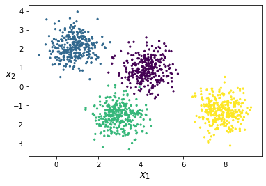
Figure 3: Spherical data blobs

But these clusters are all spherical and too easy to differentiate that relatively simpler (and popular) algorithm such as K-means are able to perform really well. What K-means is not good at is in the cases where the clusters are non-spherical in shape. K-means lacks flexibility when it comes to determining the shape of clusters. Another disadvantage is that it lacks probabilistic cluster assignments. These two disadvantages are readily addressed in GMM. And also, instead of using these spherical clusters, we’ll stretch them. This is what the later two lines in the above code snippet do. The figure below shows the data we will be using henceforth.

Figure 4: Stretched data blobs

Now, to apply the GMM on this dataset that we have just created, we’ll first create an instance of GaussianMixture class available in the sklearn.mixture package as follows:

gm = GaussianMixture(n_components=4, n_init=10, random_state=42)

Note that n_components hyperparameter is used to define the number of mixture components i.e. number of clusters K which in our case is set to 4. n_init=10 simply means that the parameters of the model will be initialized 10 times and the best one will be kept as the result. The default value for this parameter is 1. Now, we can train this model on the data as:

gm.fit(X)

We’ll get the following output once the model has been fitted with our data:

Figure 5: Output after fitting the model

Notice the very first hyperparameter covariance_type? This hyperparameter is used to set constraints on the shape, size, and orientation of the clusters. By default, it is set to 'full' which means each cluster can be of any form i.e. it can have its own unconstrained covariance matrix. Other options for this hyperparameter are:

• 'spherical': Clusters must be spherical but can have different diameters i.e. different variances.

• 'diag': Clusters can take any shape, but ellipsoid’s axes must be parallel to the coordinate axes. The covariance matrix must be diagonal.

• 'tied': All clusters must have the same ellipsoidal shape, size, and orientation. All clusters share the same covariance matrix.

Once the model has been trained, we can get the parameter values for the different clusters using the attributes means_, covariances_ and weights_ for means µ(j), covariance matrices Σ(j), and cluster probabilities ϕʲ respectively for j ∈ {1, ..., K}.

The arrays of means, covariance matrices, and cluster probabilities (in order from top to bottom) are given as follows:

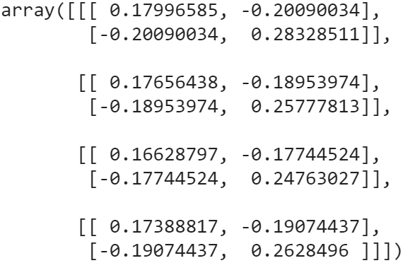
Further, we can confirm whether the model has converged or not using converged_ attribute, and to check the number of iterations it took our model to converge, we can use n_iter_. Values for these attributes in our case have come out to be True and 6 respectively. Now let’s see how the decision boundaries computed by the model looks like.

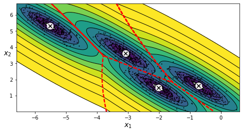
Figure 6: Decision boundaries

Looks pretty good. And even though the clusters are not very obviously spherical but still if we had set the covariance_type_=“spherical” then the resultant decision boundaries would have looked something like this:

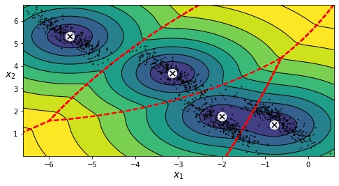
Figure 7: Decision boundaries when covariance_type_='spherical'

This looks so bad that the decision boundaries represented by red dots are cutting right through the original blobs. Up until now, we have been seeing that for clustering to be performed, we have to explicitly define the value of K. But there would certainly be cases where we would not have prior knowledge of what the actual number of clusters are so… HOW DO WE SELECT THE VALUE FOR K?

For algorithms such as K-Means, we are able to use metrics such as inertia and silhouette score to get the appropriate value for K but as it turns out, we cannot use these same metrics for GMMs. Apparently, these metrics are not reliable when the clusters are non-spherical and different in sizes. So, instead what we do is we try to find a model that would minimize a theoretical information criterion. Two such criteria are the Bayesian information criterion (BIC) and the Akaike information criterion (AIC). Both of these are defined as:

Here, p is the number of parameters learned by the model. Both of these criteria penalize the models that have more parameters to learn and reward the model that fits well on the data. Although most of the time we’ll see that model selected using both the criteria is more or less the same, but when they differ, model selected using BIC tends to be simpler (fewer parameter) and weaker fit on the data as compared to AIC. We can get these values for the model in Scikit-Learn very easily by just calling the methods bic() and aic() on the model’s instance.

Then to find the appropriate value for K, we can train multiple models with varying values for the hyperparameter n_components and finally select the model that gives the lowest value for the information criterion. We can do so as follows:

gms_per_k = [GaussianMixture(n_components=k, n_init=10,                 random_state=42).fit(X)for k in range(1, 11)] 
bics = [model.bic(X_stretched) for model in gms_per_k] 
aics = [model.aic(X_stretched) for model in gms_per_k]

Let’s now plot the values for bics and aics w.r.t. K:

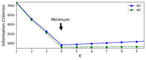
Clearly, both the information criteria are at their lowermost values when K = 4 which is also the value we selected while generating our data. Hence, these criteria will mostly work just fine for selecting the values of K. Note that, the same criteria can also be used to select the best values for other hyperparameters of the model as well. The only downside to this method is that we have to train multiple models in order to determine the appropriate values which can quickly become computationally expensive as the size and dimensionality of our data increases. Side note: There’s a more powerful variant that can help us automate the process of selecting the optimal value for K: Bayesian Gaussian mixture models. We’ll discuss it sometime later. For now, let’s end our discussion with some applications of GMMs. APPLICATIONS

• GMMs have been used for feature extraction such as in speech recognition systems.

• GMMs are applied to high-dimensional data to reduce the number of dimensions and still preserving useful information.

• GMMs have also been used in object tracking of multiple objects, where the number of mixture components and their means predict object locations at each frame in a video sequence.

REFERENCES AND ADDITIONAL RESOURCES

• Hands-On Machine Learning with Scikit-Learn, Keras, and Tensor Flow: Concepts, Tools, and Techniques to Build Intelligent Systems.

• Deep Learning Book.

• Clustering (4): Gaussian Mixture Models and EM

• https://brilliant.org/wiki/gaussian-mixture-model/